
Data, data everywhere! Our apps collect information from any kind of service and produce new data themselves. Data that need to be stored and then? A grid, an Excel report, some plot: that’s what we usually do with them. As developers, we stop to the button “Save as Excel” trying to find a clever way to map our sophisticated domain objects into this archaic and flattening format where everything is put on a row, repeated millions of times.
There is a mantra repeated everywhere: the more data we have, the best we can analyze them to find hidden patterns bringing to the solution of real problems. Unfortunately, these patterns are too much complex to be found by human eyes. This is exactly what Machine Learning does: it examines large amounts of data looking for patterns, then generates code that lets you recognize those patterns in new data. The goal is to get back to our apps and make them smarter. For example, we want to predict failures on an assembly line or to find malwares in our e-mail.
It sounds fantastic, but if you ask around it seems that Machine Learning is like a programmable washing machine. You throw the dirty laundry (the data) inside it, choose a cycle, add some detergents, turn on, go around for a while, come back and… voilà your Model is ready! “Did you add some neural networks? Next time, a little bit more!”
The full process is shown in this threatening and complex picture (source: Introducing Azure Machine Learning)

“You just need to know a little bit of statistical techniques to analyze data”. This is the second naive assumption you’ll hear around. Everyone knows how to calculate an average (right?) but very few people remember the Bayes’ theorem.
Once the idea to go back to the books is accepted, we face a third problem. Every training course shows dataset analyzing classical problems: the taxi tips in New York, the flat price per square meter, the correlation between the weight of an unborn child and the data available about the mother. The model creation flows in a very smooth way, like a washing machine cycle. But when we pass to our data, everything seems to make no sense at all.
The Internet is full of articles speaking about bizarre correlations (look here).). The most interesting is the one claiming that developers who use spaces make more money than those who use tabs (a more in-depth analysis of this data by Evelina Gabasova is available here) .

The starting point of this article (and the next ones) will be some data collected in the last few months concerning football matches and players.
We want to focus on data pre-processing: all that we need to create clean and optimized datasets, to be passed to the famous algorithms producing predictive models to be used on new data.
We’ll start from a file containing in each row the following information related to a football match played by a single player:

In details, we have the player’s age in the day of the match, how many minutes he played, his role (for example DC is a centre-back), the match result, the teams involved, number of goals, assists, own-goals. etc.
Are these data (originating from a simple scraping of html pages) valid? Are they suitable for a statistical analysis?
I’ll use a cloud service, Azure Machine Learning, to try to understand it. Why we need to use it? Because we need some help with a lot of trivial but time-consuming tasks. The starting address is the following: https://studio.azureml.net
Once registered, we meet the following dashboard:

We can upload a dataset in .csv format from a local file on our pc.


Once uploaded a dataset on the portal, we can create a Jupyter notebook to study it. It’s an interactive interface for data analysis based on an open source standard. With Azure portal, you can choose between R, Python 2 or Python 3 as languages to insert commands. I choose R.

The head command shows the first few rows of our dataset. If you type summary (name of the dataset variable), a statistical summary is shown in each column.
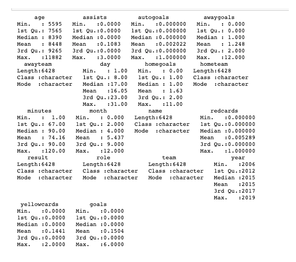
Some data make sense. For example, year values are in a range of 2006-2019. minutes range is from 1 to 120 (some matches extended to overtime). age range is from 15,3 to a maximum of 32,55. The month column has a 0 minimum value while it should vary between 1 and 12. We found a typical bug in the data extraction that need to be corrected.
Some columns have no meaning at all from the statistical perspective. For example, result is a property assuming three possible values: W (win), L (loss), D (deuce). We say that result is a categorical feature. Most of machine learning algorithms expect numerical values as input.
We need to transform result in a numerical property. The most used technique is called one-hot encoding. Rather than replacing the categorical value with an arbitrary numeric one, we define three new numerical variables. Let’s call them is_win, is_loss, is_deuce. Each of them will assume a value that will be 0 or 1.
The same procedure will be applied to the player’s role. Unfortunately, there are only 12 roles, causing a rather tedious normalization. In these articles, we’ll focus just on three roles: is_defender, is_midfield and is_forward. The role normalization showed that we don’t have data about the goalkeepers. Besides, in several rows, the data about the role is missing.
There isn’t a standard formula to manage missing data because the solution depends on the context and how data were extracted. You could simply fully remove the rows as soon they have missing values on a column. This solution is not very popular because you risk losing a lot of data and because the loss of data could hide a pattern.
Another technique is the one replacing null values with our best estimate. In our case, if we could query a database, we could extract the typical player’s role and replace the missing data. I choose simply to add a new property called is_norole.
As you can see, a simple example could hide pitfalls and it might make us make decisions we may come to regret. Data are never perfect!
The name property showing the player’s name probably makes no sense unless you are not interested in analyzing the player’s career (but this is more a data visualization problem). I choose also to remove the team names, leaving only the information about the player belonging or not to the home team (is_home with two possible values: 0 or 1).
Machine Learning algorithms benefit from numerical values normalization, ranging in a well-known range. For example, minutes could be expressed as a number ranging between 0 and 1, dividing it by 120 (the maximal match duration). We applied the same procedure to age, dividing it by 16425 (number obtained multiplying 45 years by 365 days): another choice!
The final result of our first attempt of data normalization can be loaded again on Azure Machine Learning Studio.


We can now load the data regarding other teams. All the files can be found in the following Github repository: https://github.com/sorrentmutie/FootballDataForMachineLearning
In total, we have 50770 rows. Are they enough? Can we “load the washing machine”? As developers, we use the term properties while in machine learning we define them as features. Do we have good features? When a feature can be defined as good? The answer is in the following five points:
- the feature must be related to the objective;
- it must be known at prediction time;
- it must be numeric with meaningful magnitude;
- we should have enough examples;
- we must bring human insight in the problem.
As you could easily realize, there is still a long way to go. Today, we stop here, and we’ll continue our journey in the next post.